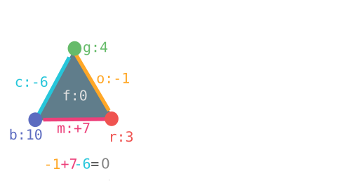
Once again, we have our humble triangle with vertices $V = \{r, g, b\}$, edges $E = \{o, m, c \}$, faces $F = \{ f \}$ with boundary maps $\partial_{EV}$, $\partial_{FE}$:

• $\partial_{FE}(f)= o + m + c$
• $\partial_{EV}(o) = r - g$
• $\partial_{EV}(m) = b - r$
• $\partial_{EV}(c)= g - b$

We define a function $h_v: V \rightarrow \mathbb R$ on the vertices as:

• $h_v(r) = 3$, $h_v(g) = 4$, $h_v(b) = 10$.

We now learn how to extend this function to the higher dimensional objects, the edges and the faces of the triangle.

To extend this function to the edges, we define a new function:

• $h_e: E \rightarrow R$
• $h_e(e) \equiv \sum_i \alpha_i h_v(v_i)$ where $\partial_{EV} e = \sum_i \alpha_i v_i$

Expanded out on the example, we evaluate $h_v$ as:

• $h_e(o) \equiv d h_v(o) = h_v(r) - h_v(g) = 3 - 4 = -1$
• $h_e(m) \equiv d h_v(m) = h_v(b) - h_v(r) = 10 - 3 = +7$
• $h_e(c) \equiv d h_v(c) = h_v(g) - h_v(b) = 4 - 10 = -6$

More conceptually, we have created an operator called $d$ (the coboundary operator ) which takes functions defined on vertices to functions defined on edges. This uses the boundary map on the edges to "lift" a function on the vertices to a function on the edges. It does so by assigning the "potential difference" of the vertices to the edges.

• $d: (V \rightarrow \mathbb R) \rightarrow (E \rightarrow \mathbb R)$
• $d(h_v) \equiv h_e$, $h_e(e) \equiv \sum_i \alpha_i f(v_i)$ where $\partial_{EV} e = \sum_i \alpha_i v_i$

We can repeat the construction we performed above, to construct another operator $d : (E \rightarrow \mathbb R) \rightarrow (F \rightarrow \mathbb R)$, defined in exactly the same way as we did before. For example, we can evaluate:

• $h_f \equiv d(h_e)$
• $h_f(f) \equiv d h_e(f) = h_e(o) + h_e(m) + h_e(c) = -1 + 7 -6 = 0$

What we have is a chain:

• $h_v \xrightarrow{d} h_e \xrightarrow{d} h_f$

Where we notice that $d^2 = d \circ d = 0$, since the function $h_f$ that we have gotten evaluates to zero on the face $f$. We can prove this will happen in general , for any choice of $h_v$. (it's a good exercise in definition chasing).

Introducing some terminology, A differential form $f$ is said to be a closed differential form iff $df = 0$.

In our case, $h_e$ is closed , since $d h_e = h_f = 0$. On the other hand $h_v$ is not closed , since $d h_v = h_e \neq 0$.

The intuition for why this is called "closed" is that its coboundary vanishes.

§ Exploring the structure of functions defined on the edges

Here, we try to understand what functions defined on the edges can look like, and their relationship with the $d$ operator. We discover that there are some functions $g_e: E \rightarrow \mathbb R$ which can be realised as the differential of another function $g_v: V \rightarrow \mathbb R$. The differential forms such as $g_e$ which can be generated a $g_v$ through the $d$ operator are called as exact differential forms . That is, $g_e = d g_v$ exactly , such that there is no "remainder term" on applying the $d$ operator.

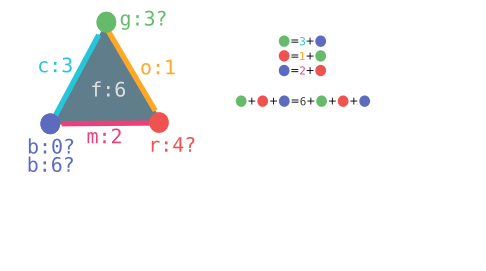
We take an example of a differential form that is not exact , which has been defined on the edges of the triangle above. Let's call it $h_e$.

It is defined on the edges as:

• $h_e(c) = 3$
• $h_e(m) = 2$
• $h_e(o) = 1$

We can calcuate $h_f = d h_e$ the same way we had before:

• $h_f(f) \equiv d h_e(f) = h_e(o) + h_e(m) + h_e(c) = 3 + 1 + 2 = 6$.

Since $d h_e \neq 0$, this form is not exact.

Let's also try to generate $h_e$ from a potential. We arbitrarily fix the potential of $b$ to $0$. That is, we fix $h_v(b) = 0$, and we then try to see what values we are forced to values of $h_v$ across the rest of the triangle.

• $h_v b = 0$
• $h_e(c) = h_v(g) - h_v(b)$. $h_v(g) = h_v(b) + h_e(c) = 0 + 3 = 3$.
• $h_e(o) = h_v(r) - h_v(g)$. $h_v(r) = h_v(g) + h_e(o) = 3 + 1 = 4$.
• $h_e(m) = h_v(b) - h_v(r)$ $2 = 0 - 4$. This is a contradiction!
• Ideally, we need $h_v(b) = 6$ for the values to work out.

Hence, there can exist no such $h_v$ such that $h_e \equiv d h_v$. The interesting thing is, when we started out by assigning $h_v(b) = 0$, we could make local choices of potentials that seemed like they would fit together, but they failed to fit globally throughout the triangle. This failure of locally consistent choices to be globally consistent is the essence of cohomology.

§ Cohomology of half-filled butterfly

Here, we have vertices $V \equiv \\{ r, g, b, b, p \\}$, edges $E \equiv \\{rb, gr, bg, m, o, c \\}$ and faces $F \equiv \\{ f \\}$.

Here, we see a differential form $h_e$ that is defined on the edges, and also obeys the equation $dh_e = 0$ (Hence is closed). However, it does not have an associated potential energy to derive it from. That is, there cannot exist a certain $h_v$ such that $d h_v = h_e$.

So, while every exact form is closed, not every closed form is exact.

Hence, this $g$ that we have found is a non-trivial element of $Kernel(d_{FE}) / Image(d_{EV})$, since $dh_e = 0$, hence $h_e \in Kernel(d_{FE})$, while there does not exist a $h_v$ such that $d h_v = h_e$, hence it is not quotiented by the image of $d_{EV}$.

So the failure of the space to be fully filled in (ie, the space has a hole), is measured by the existence of a function $h_e$ that is closed but not exact!

This reveals a deep connection between homology and cohomology, which is made explicit by the Universal Coefficient Theorem