We have a system we wish to simulate using hamilton's equations:

We want to simulate a system using these differential equations. We will begin with some initial position and momentum $(q_0, p_0)$, evaluate $\frac{\partial q}{\partial t} \rvert_{(q_0, p_0)}$, $\frac{\partial p}{\partial t} \rvert_{(q_0, p_0)}$, and use these to find $(q_{next}, p_{next})$. An integrator is a general algorithm that produces the next position and momentum using current information:

The design of $I$ is crucial: different choices of $I$ will have different trade-offs for accuracy and performance. Another interesting property we might want is for $I$ to be a symplectic integrator --- that is, it preserves the total energy of the system. For example, here's a plot of the orbits of planets using two integrators, one that's symplectic (leapfrog) and one that isn't (Euler)

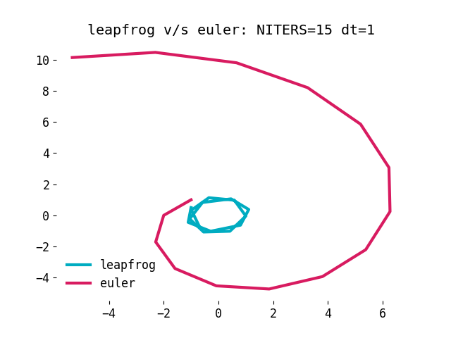
Notice that since leapfrog attempts to keep energy conserved, the orbits stay as orbits! On the other hand, the euler integrator quickly spirals out, since we lose energy during the integration. Note that this is not an issue of numerical precision : The euler integrator is ineherently such that over long timescales, it will lose energy. On the other hand, the leapfrog integrator will always remain stable , even with very large timesteps and low precision.

I present the equations of the leapfrog integrator, a proof sketch that it is symplectic, and the code listing that was used to generate the above plot. Often, code makes most ideas very clear!

§ The integrator

§ Code listing

§ Incantations

# Run HMC with a particular choice of potentialimport numpy as npfrom matplotlib.animation import FuncAnimationimport matplotlib.pyplot as pltimport numpy.linalg

# dq/dt = dH/dp|_{p0, q0}# dp/dt = -dH/dq|_{p0, q0}def leapfrog(dhdp, dhdq, q0, p0, dt):    p0 += -dhdq(q0, p0) * 0.5 * dt    # full step position    # q += dt * p    q0 += dhdp(q0, p0) * dt    # half step position    p0 += -dhdq(q0, p0) * 0.5 * dt    return (q0, p0)

For reference, we also implement an euler integrator, that uses the derivative to compute the position and momentum of the next timestep independently.

def euler(dhdp, dhdq, q, p, dt):    pnew = p + -dhdq(q, p) * dt    qnew = q + dhdp(q, p) * dt    return (qnew, pnew)

Finally, we implement planet(integrator, n, dt) which simulates gravitational potential and usual kinetic energy, using the integrator given by integrator for n steps, with each timestep taking dt.

def planet(integrator, n, dt):    STRENGTH = 0.5    # minimise potential V(q): q, K(p, q) p^2    q = np.array([0.0, 1.0])    p = np.array([-1.0, 0.0])    # H = STRENGTH * |q| (potential) + p^2/2 (kinetic)    def H(qcur, pcur): return STRENGTH * np.linalg.norm(q) + np.dot(p, p) / 2    def dhdp(qcur, pcur): return p    def dhdq(qcur, pcur): return STRENGTH * 2 * q / np.linalg.norm(q)    qs = []    for i in range(n):        print("q: %10s | p: %10s | H: %6.4f" % (q, p, H(q, p)))        (q, p) = integrator(dhdp, dhdq, q, p, dt)        qs.append(q.copy())    return np.asarray(qs)

We plot the simulations using matplotlib and save them.

NITERS = 15TIMESTEP = 1print("planet simulation with leapfrog")planet_leapfrog = planet(leapfrog, NITERS, TIMESTEP)plt.rcParams.update({'font.size': 12, 'font.family':'monospace'})fig, ax = plt.subplots()print(planet_leapfrog)ax.plot(planet_leapfrog[:, 0], planet_leapfrog[:, 1], label='leapfrog',        linewidth=3, color='#00ACC1')print("planet simulation with euler")planet_euler = planet(euler, NITERS, TIMESTEP)ax.plot(planet_euler[:, 0], planet_euler[:, 1], label='euler',        linewidth=3, color='#D81B60')legend = plt.legend(frameon=False)ax.set_title("leapfrog v/s euler: NITERS=%s dt=%s" % (NITERS, TIMESTEP))ax.spines['top'].set_visible(False)ax.spines['right'].set_visible(False)ax.spines['bottom'].set_visible(False)ax.spines['left'].set_visible(False)plt.savefig("leapfrog-vs-euler.png")plt.show()